Landscape Portal

An open-method geostory

Reading the riverbank

How terrain turns a fixed distance into a question we can inspect, map and challenge.

Begin the story

A line beside water can look final on a map. In practice, it is the end of a chain of choices: which water objects count, what width to test, and where the land is steep enough to change the result.

I wanted to make that chain visible. This story follows one real test area from a one-metre elevation model and 52 mapped water features to a reproducible screening result.

The map does not establish a legal boundary. It shows a transparent protocol: the inputs, assumptions and outputs stay available for inspection and download.

A spatial rule becomes useful for public discussion when its assumptions can be seen—not hidden behind the final polygon.
5.457km² study area
1 mterrain resolution
52water features
slope test

The landscape, layer by layer

Scene 1 / 6

Riparian protective-strip screening map A scroll-driven map of terrain, water objects, a standard screening zone and slope-triggered extensions.
Water 50 m zone Extension to 100 m
Loading the case-study layers…

01

Begin with terrain

The land is not a flat buffer

Across this compact test area, elevation changes from 128 to 216 metres. The one-metre DEM lets the method examine those changes close to the shoreline.

Scroll over the map to zoom; drag to pan after zooming. Select a coloured zone for details.

02

Map the evidence

Water is a network, not one line

The source contains 42 polygonal and 10 linear water features. Their geometry becomes the common reference from which distance and terrain are measured.

42 + 10polygon and line features

03

Expose the parameter

First, test a visible 50-metre width

The source attributes do not legally classify each water object. I therefore use 50 metres as an explicit test setting, not as a claim about the correct statutory width for every feature.

0.756 km²standard screening area

04

Read the slope

Extend only where the terrain test triggers

At the 50 m ring, the method compares terrain height with the nearest shoreline. Shoreline pixels linked to a slope above 3° extend the analytical band toward 100 metres.

1,709flagged shoreline pixels

05

See the difference

The extension is selective

The rust-coloured areas are not a second uniform buffer. They appear only where the terrain condition is met, adding 0.411 km² to the screening picture.

0.411 km²terrain-triggered extension

06

Keep the protocol open

A result should carry its evidence

The archive, individual inputs, derived layers, QGIS model, theory note, metadata, checksums and reproducibility script are published together. The map is an entry point, not a sealed conclusion.

Open the GitHub source →
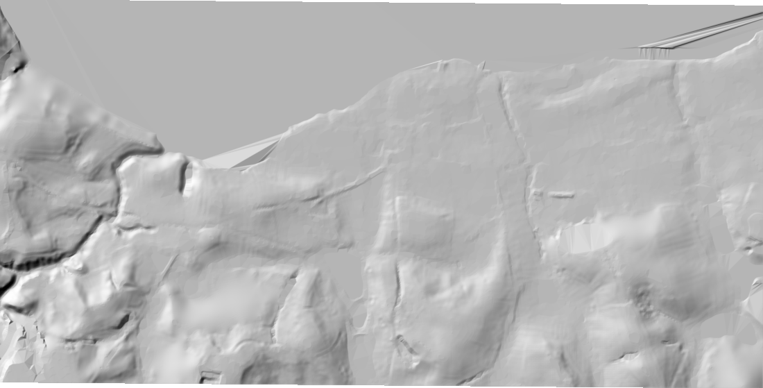
Shaded elevation model used in the case study
The source surface One metre per pixel The terrain image is derived from the downloadable DEM. Light and shadow make the local relief legible, but the analysis uses elevation values—not the illustration.

From rule to repeatable operations

The method is a sequence, not a magic polygon

  1. 01Prepare

    Align the DEM, water geometry and analysis extent in a projected CRS.

  2. 02Measure

    Create the 50 m test ring and associate terrain cells with the nearest shoreline.

  3. 03Test

    Compare elevation change and distance to identify slopes above 3°.

  4. 04Publish

    Export the standard zone, extensions, metadata and reproducibility materials.

What the map adds

The visible output is only half the point

A transparent workflow lets someone else distinguish data from assumptions, rerun the analysis with another parameter, and argue about the method with the same evidence in view.

Continue with the evidence

Inspect the data. Reproduce the method.

Version 1.0.0 keeps source data, results, documentation and checksums together. Choose the complete package or go to the resource record for individual files.